Overkill Analytics

This website’s goal is to develop and explain a data science philosophy – overkill analytics – that leverages computing scale and rapid development technologies to produce faster, better, and cheaper solutions to predictive modeling problems.   To achieve this goal, one core question must be answered: when attacking data science problems, how can we use CPU as a substitute for IQ?   This post will discuss the fundamental ‘overkill’ weapon for addressing this question – ensemble learning.

Ensembles are nothing new, of course; they underlie many of the most popular machine learning algorithms (e.g., random forests and generalized boosted models) .   The theory is that consensus opinions from diverse modeling techniques are more reliable than potentially biased or idiosyncratic predictions from a single source.    More broadly, this principle is as basic as “two heads are better than one.”   It’s why cancer patients get second opinions, why the Supreme Court upheld affirmative action, why news organizations like MSNBC and Fox hire journalists with a wide variety of political leanings…

Well, maybe the principle isn’t universally applied.   Still, it is fundamental to many disciplines and holds enormous value for the data scientist.   Below, I will explain why, by addressing the following:

• Ensembles add value: Using ‘real world’ evidence from Kaggle and GigaOM‘s recent WordPress Challenge, I’ll show how very basic ensembles – both within my own solution and, more interestingly, between my solution and the second-place finisher – added significant improvements to the result.
• Why ensembles add value:  For the non-expert (like me), I’ll give a brief explanation of why ensembles add value and support overkill analytics’ chief goal: leveraging computing scale productively.
• How ensembles add value: Also for the non-expert, I’ll run through a ‘toy problem’ depiction of how a very simple ensemble works, with some nice graphs and R code if you want to follow along.

Most of this very long post may be extremely rudimentary for seasoned statisticians, but rudimentary is the name of the game at Overkill Analytics.   If this is old hat for you, I’d advise just reading the first section – which has some interesting real world results – and glancing at the graphs in the final section (which are very pretty and are useful teaching aids on the power of ensemble methods).

Ensembles Add Value: Two Data Geeks Are Better Than One

Overkill analytics is built on the principle that ‘more is always better’.   While it is exciting to consider the ramifications of this approach in the context of massive Hadoop clusters with thousands of CPUs, sometimes overkill analytics can require as little as adding an extra model when the ‘competition’ (a market rival, a contest entrant, or just the next best solution) uses only one.   Even more simply, overkill can just mean leveraging results from two independent analysts or teams rather than relying on predictions from a single source.

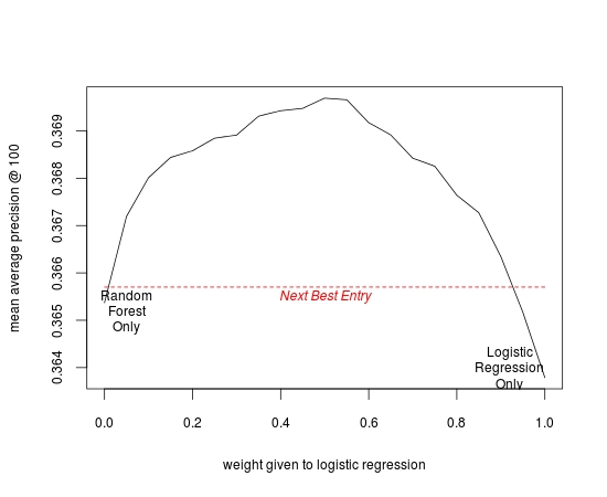
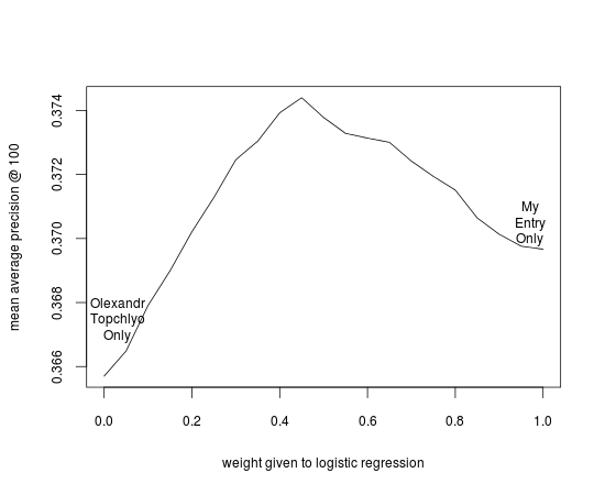
Below is some evidence from my recent entry in the WordPress Challenge on Kaggle.   (Sorry to again use this as an example, but I’m restricted from using problems from my day job.).  In my entry, I used a basic ensemble of a logistic regression and a random forest model – each with essentially the same set of features/inputs – to produce the requested recommendation engine for blog content.   From the chart below, you can see how this ensemble performed in the evaluation metric (mean average precision @ 100) at various ‘weight values’ for the ensemble components:

Note that either model used independently as a recommendation engine – either a random forest solution or a logistic regression solution – would have been insufficient to win the contest.   However, taking an average of the two produced a (relatively) substantial margin over the nearest competitor.   While this is a fairly trivial example of ensemble learning, I think it is significant evidence of the competitive advantages that can be gained from adding just a little scale.

For a more interesting example of ensemble power, I ran the same analysis with an ensemble of my recommendation engine and the entry of the second place finisher (Olexandr Topchylo).    To create the ensemble, I used nothing more complicated than a ‘college football ranking’ voting scheme (officially a Borda count):  assign each prediction a point value equal to its inverse rank for the user in questions.   I then combined the votes at a variety of different weights, re-ranked the predictions per user, and plotted the evaluation metric:

By combining the disparate information generated by my modeling approach and Dr. Topchlyo’s, one achieves a predictive result superior to that of any individual participant by 1.2% – as large as the winning margin in the competition.   Moreover, no sophisticated tuning of the ensemble is required – a 50/50 average comes extremely close to the optimal result.

Ensembles are a cheap and easy technique that allows one to combine the strengths of disparate data science techniques or even disparate data scientists.  Ensemble learning showcases the real power of Kaggle as a platform for analytics – clients receive not only the value of the ‘best’ solution, but also the superior value of the combined result.   It can even be used as a management technique for data science teams (e.g., set one group to work collaboratively on a solution, set another to work independently and combine results in an ensemble, and compare – or combine – the results of the two teams).   Any way you slice it, the core truth is apparent:  two data geeks are always better than one.

Why Ensembles Add Value:  Overkilling Without Overfitting

So what does this example tell us about how ensembles can be used to leverage large-scale computing resources to achieve faster, better, and cheaper predictive modeling solutions?   Well, it shows (in a very small way) that computing scale should be used to make predictive models broader rather than deeper.   By this, I mean that scale should be used first to expand the variety of features and techniques applied to a problem, not to delve into a few sophisticated and computationally intensive solutions.

The overkill approach is to abandon sophisticated modeling approaches (at least initially) in favor of more brute force techniques.  However, unconstrained brute force in predictive modeling is a recipe for disaster.   For example, one could just use extra processing scale to exhaustively search a function space for the model that best matches available data, but this would quickly fail for two reasons:

• exhaustive searches of large, unconstrained solution spaces are computationally impossible, even with today’s capacity; and
• even when feasible, searching purely on the criteria of best match will lead to overfit solutions: models which overlearn the noise in a training set and are therefore useless with new data.

At the risk of overstatement, the entire field of predictive modeling (or data science, if you prefer) is to address these two problems – i.e., to find techniques which search a narrow solution space (or narrowly search a large solution space) for productive answers, and to find search criteria that discover real solutions rather than just learning noise.

So how can we overkill without the overfit?   That’s where ensembles come in.   Ensemble learning uses combined results from multiple different models to provide a potentially superior ‘consensus’ opinion.   It addresses both of the problems identified above:

• Ensemble methods have broad solution spaces (essentially ‘multiplying’ the component search spaces) but search them narrowly – trying only combinations of ‘best answers’ from the components.
• Ensembles methods avoid overfitting by utilizing components that read irrelevant data differently (canceling out noise) but read relevant inputs similarly (enhancing underlying signals).

It is a simple but powerful idea, and it is crucial to the overkill approach because it allows the modeler to appropriately leverage scale: use processing power to create large quantities of weak predictors which, in combination, outperform more sophisticated methods.

The key to ensemble methods is selecting or designing components with independent strengths and a true diversity of opinion.     If individual components add little information, or if they all draw the same conclusion from the same facts, the ensemble will add no value and even reinforce errors from individual components.   (If a good ensemble is like a panel of diverse musical faculty using different criteria to select the best students for Juliard, a bad ensemble would be like a mob of tween girls advancing Sanjaya on American Idol.)   In order to succeed, the ensemble’s components must excel at finding different types of signals in your data while having varied, uncorrelated responses to your data’s noise.

How Ensembles Add Value:  A Short Adventure In R

As shown in the first section of this post, a small but effective example of ensemble modeling is to take an average of classification results from a logistic regression and a random forest.   These two techniques are good complements for an ensemble because they have very different strengths:

• Logistic regressions find broad relationships between independent variables and predicted classes, but without guidance they cannot find non-linear signals or interactions between multiple variables.
• Random forests (themselves an ensemble of classification trees) are good at finding these narrower signals, but they can be overconfident and overfit noisy regions in the input space.

Below is a walkthrough applying this ensemble to a toy problem – finding a non-linear classification signal from a data set containing the class result, the two relevant inputs, and two inputs of pure noise.

The signal for our walk-through is a non-linear equation of two variables dictating the probability of vector X belongs to a class C:

The training data uses the above signal to determine class membership for a sample of 10,000 two-dimensional X vectors (x1 and x2).  The dataset also includes two irrelevant random features (x3 and x4) to make the task slightly more difficult.   Below is R code to generate the training data and produce two maps showing the signal we are seeking as well as the training data’s representation of that signal:

# packages
require(fields) # for heatmap plot with legend
require(randomForest) # requires installation, for random forest models
random.seed(20120926)
# heatmap wrapper, plotting func(x, y) over range a by a
hmap.func <- function(a, f, xlab, ylab) 
{
	image.plot(a, a, outer(a, a, f), zlim = c(0, 1), xlab = xlab, ylab = ylab)
}
# define class signal
g <- function(x, y) 1 / (1 + 2^(x^3+ y+x*y))
# create training data
d <- data.frame(x1 = rnorm(10000), x2 = rnorm(10000)
				,x3 = rnorm(10000), x4 = rnorm(10000))
d$y = with(d, ifelse(runif(10000) < g(x1, x2), 1, 0))
# plot signal (left hand plot below)
a = seq(-2, 2, len = 100)
hmap.func(a, g, "x1", "x2")
# plot training data representation (right hand plot below)
z = tapply(d$y,  list(cut(d$x1, breaks = seq(-2, 2, len=25))
				 , cut(d$x2, breaks = seq(-2, 2, len=25))), mean)
image.plot(seq(-2, 2, len=25), seq(-2, 2, len=25), z, zlim = c(0, 1)
			, xlab = "x1", ylab = "x2")

Signal In x1, x2	Training Set in x1, x2

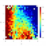As you can see, the signal is somewhat non-linear and is only weakly represented by the training set data.   Thus, it presents a reasonably good test for our sample ensemble.

The next batch of code and R maps show how each ensemble component, and the ensemble itself, interpret the relevant features:

# Fit log regression and random forest
fit.lr = glm(y~x1+x2+x3+x4, family = binomial, data = d)
fit.rf = randomForest(as.factor(y)~x1+x2+x3+x4, data = d, ntree = 100, proximity = FALSE)
# Create funtions in x1, x2 to give model predictions
# while setting x3, x4 at origin
g.lr.sig = function(x, y) predict(fit.lr, data.frame(x1 = x, x2 = y, x3 = 0, x4 = 0), type = "response") 
g.rf.sig = function(x, y) predict(fit.rf, data.frame(x1 = x, x2 = y, x3 = 0, x4 = 0), type = "prob")[, 2] 
g.en.sig = function(x, y) 0.5*g.lr.sig(x, y) + 0.5*g.rf.sig(x, y)
# Map model predictions in x1 and x2
hmap.func(a, g.lr.sig, "x1", "x2")
hmap.func(a, g.rf.sig, "x1", "x2")
hmap.func(a, g.en.sig, "x1", "x2")

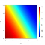
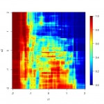
Log. Reg. in x1, x2	Rand. Forest In x1, x2	Ensemble in x1, x2

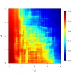Note how the logistic regression makes a consistent but incomplete depiction of the signal – finding the straight line that best approximates the answer.   Meanwhile, the random forest captures more details, but it is inconsistent and ‘spotty’ due to its overreaction to classification noise.   The ensemble marries the strengths of the two, filling in some of the ‘gaps’ in the random forest depiction with steadier results from the logistic regression.

Similarly, ensembling with a logistic regression helps wash out the random forest’s misinterpretation of irrelevant features.   Below is code and resulting R maps showing the reaction of the models to the two noisy inputs, x3 and x4:

# Create funtions in x3, x4 to give model predictions
# while setting x1, x2 at origin
g.lr.noise = function(x, y) predict(fit.lr, data.frame(x1 = 0, x2 = 0, x3 = x, x4 = y), type = "response")
g.rf.noise = function(x, y) predict(fit.rf, data.frame(x1 = 0, x2 = 0, x3 = x, x4 = y), type = "prob")[, 2] 
g.en.noise = function(x, y) 0.5*g.lr.noise(x, y) + 0.5*g.rf.noise(x, y)
# Map model predictions in noise inputs x3 and x4
hmap.func(a, g.lr.noise, "x3", "x4")
hmap.func(a, g.rf.noise, "x3", "x4")
hmap.func(a, g.en.noise, "x3", "x4")

Log. Reg. Prediction in x3, x4	Rand. Forest Prediction In x3, x4	Ensemble Prediction in x3, x4

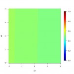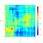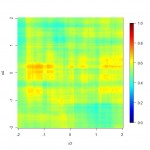As you can see, the random forest reacts relatively strongly to the noise, while the logistic regression is able to correctly disregard the information.   In the ensemble, the logistic regression cancels out some of the overfitting from the random forest on the irrelevant features, making them less critical to the final model result.

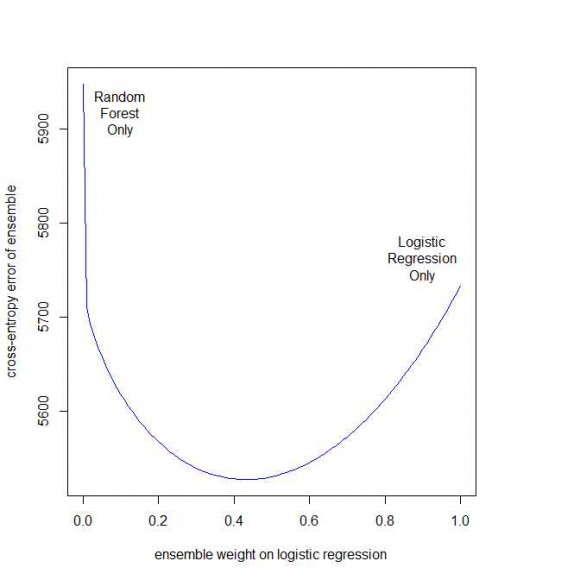
Finally, below is R code and a plot showing a classification error metric (cross-entropy error) on a validation data set for various ensemble weights:

# (Ugly) function for measuring cross-entropy error
cross.entropy <- function(target, predicted)
{
	predicted = pmax(1e-10, pmin(1-1e-10, predicted))
	- sum(target * log(predicted) + (1 - target) * log(1 - predicted))
}
# Creation of validation data
dv <- data.frame(x1 = rnorm(10000), x2 = rnorm(10000)
				, x3 = rnorm(10000), x4 = rnorm(10000))
dv$y = with(dv, ifelse(runif(10000) < g(x1, x2), 1, 0))
# Create predicted results for each model
dv$y.lr <- predict(fit.lr, dv, type = "response")
dv$y.rf <- predict(fit.rf, dv, type = "prob")[, 2]
# Function to show ensemble cross entropy error at weight W for log. reg.
error.by.weight <- function(w) cross.entropy(dv$y, w*dv$y.lr + (1-w)* dv$y.rf)
# Plot + pretty
plot(Vectorize(error.by.weight), from = 0.0, to = 1,
	xlab = "ensemble weight on logistic regression", ylab = "cross-entropy error of ensemble", col = "blue")
text(0.1, error.by.weight(0)-30, "Random\nForest\nOnly")
text(0.9, error.by.weight(1)+30, "Logistic\nRegression\nOnly")

The left side of the plot is a random forest alone, and has the highest error.   The right side is a logistic regression alone, and has somewhat lower error.   The curve shows ensembles with varying weights for the logistic regression, most of which outperform either candidate model.

Note that our most unsophisticated of ensembles – a simple average – achieves almost all of the potential ensemble gain.   This is consistent with the ‘real world’ example in the first section.   Moreover, it is a true overkill analytics result – a cheap and obvious trick that gets almost all of the benefit of a more sophisticated weighting scheme.   It also exemplifies my favorite rule of probability, espoused by poker writer Mike Caro:  in the absence of information, everything is fifty-fifty.

Super long post, I realize, but I really appreciate anyone who got this far.   I plan one more post next week on the WordPress Challenge, which will describe the full list of features I used to create the ensemble model and a brief (really) analysis of the relative importance of each.

As always, thanks for reading!